DNA-origami nanorulers

DNA-origami nanorulers are reference samples for super-resolution microscopy: a stiff DNA rod with marks placed on it to nanometre accuracy, so that a microscope's image can be checked against a known distance [scheckenbach2020]. inSiliScope's nanoruler sample is a field of such rods lying flat on the coverslip, each carrying three spots of DNA-PAINT docking strands 80 nm apart (the spacing is adjustable), or of flat 2D origami carrying a pattern of strands (the TU Delft logo). Mount it with the viewer's Specimen select, Micro-Manager's SampleHolder (or the Specimen config group) or the CLI's --specimen Nanorulers (Samples). The dyes, the light path, the PSF and the camera are the same as for the cell field (Physics).

Each molecule goes through: the design at rest → which strands carry a dye (the label) → bending → landing (roll, height) → placement (position, direction). Every step is a pure function of the seed and the molecule's address, so any window of the field can be made alone, in any order, with the same result.

The designs

The designs live in data/origami/designs.json (Design). Their spots sit on a lattice whose step is the site spacing (SpacingNm: 640, 320, 160, 80, 40, 20, 10 or 5 nm in the viewer and Micro-Manager, any value on the CLI), and the molecule grows or shrinks with it.

1D origami: the nanoruler

Nanoruler:

• Body: a cylinder 13 nm in diameter, the typical nanoruler, a 12-helix bundle [scheckenbach2020] (p. 110902-3), reaching 20 nm beyond the outer spots: 2 × spacing + 40 nm long. At the default 80 nm that is the typical 200 nm rod.
• Spots: A, B and C one spacing apart, 20 nm from the ends: at 80 nm spacing at 20, 100 and 180 nm along the rod (80 nm from A to B and from B to C, 160 nm from A to C); at 40 nm at 20, 60 and 100 nm of a 120 nm rod. A longer rod bends more (below).
• Strands: each spot is a ring of 5 docking-strand positions, 72° apart around the rod (radius 6.5 nm). This is a modelling choice, not a product's specification; no published strand count per spot was found. StrandsPerSpot (1-5) keeps positions 1..N of each ring, the same subset on every rod.

2D origami: the TU Delft logo

TUDelftLogo: a flat single-layer sheet carrying the TU Delft logo (flame, T, U and D) as 37 cells of a 17 × 11 map of flat-topped hexagons, one docking strand at the centre of each, neighbouring centres one spacing apart (columns spacing × √3/2 apart, odd columns half a step down).

• Body: a rigid plate covering the whole hex map, about 15 × 11.5 spacings (1.2 × 0.92 µm at 80 nm, 300 × 230 nm at 20 nm), 2 nm thick (about one DNA helix: estimate). It does not bend (Bending and PersistenceLengthNm do not apply).
• Landing: always face up, so the logo is never mirrored; only its direction in the plane is random. Roll does not apply.
• Strands: one per cell, on the top face (StrandsPerSpot is 1).

A new 2D design is a list of cell labels: the schema (lattice with cols, rows and cells as CCRR, column then row from the top-left, as a hex-map editor numbers them) is described at the top of designs.json and in Extending.

The spacing scales the rod and the logo alike:

The site spacing (SpacingNm). Left: a rigid nanoruler at 160, 80, 40 and 20 nm spacing, each in its own frame: the spots (A, B, C) stay one spacing apart and the rod keeps 20 nm beyond the outer ones, so it is 2 x spacing + 40 nm long. Right: the TU Delft logo 2D origami at 20 nm, a rigid plate covering its 17 x 11 hex map, one docking strand on each of the 37 logo hexagons (hollow grey: a strand left without a dye, 80 % incorporation), lying face up.

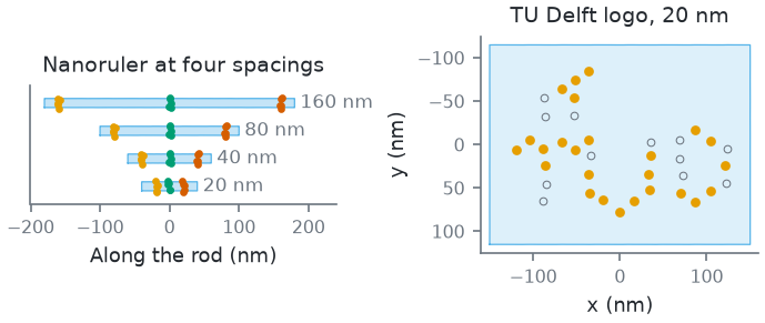
How this figure was made (5 cli runs, 14 ms)

Generated by tools/build_physics_figures.py (figure ruler-spacing) from the code it documents at commit 72b1b0f, on Linux with 4 threads, 2026-11-01. Commands, in order, with their wall time (those marked [served] ran one after the other in one insiliscope_cli --serve process, which keeps the world and the PSF kernel between commands; their outputs are the same as separate runs'):

insiliscope_cli --geometry-json rod160.geometry.json --x 0 --y 0 --specimen Nanorulers --geometry-um 4 --geometry-detail 1 --origami-spacing-nm 160 --origami-bend 0    # 4.7 ms [served]
insiliscope_cli --geometry-json rod80.geometry.json --x 0 --y 0 --specimen Nanorulers --geometry-um 4 --geometry-detail 1 --origami-spacing-nm 80 --origami-bend 0    # 2.0 ms [served]
insiliscope_cli --geometry-json rod40.geometry.json --x 0 --y 0 --specimen Nanorulers --geometry-um 4 --geometry-detail 1 --origami-spacing-nm 40 --origami-bend 0    # 1.9 ms [served]
insiliscope_cli --geometry-json rod20.geometry.json --x 0 --y 0 --specimen Nanorulers --geometry-um 4 --geometry-detail 1 --origami-spacing-nm 20 --origami-bend 0    # 1.9 ms [served]
insiliscope_cli --geometry-json logo20.geometry.json --x 0 --y 0 --specimen Nanorulers --geometry-um 4 --geometry-detail 1 --origami-design TUDelftLogo --origami-spacing-nm 20    # 3.1 ms [served]

The field

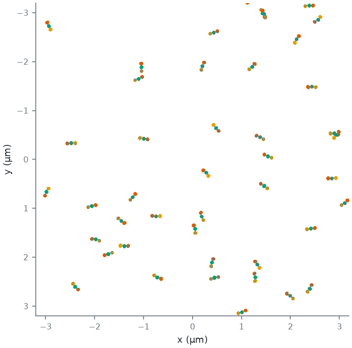
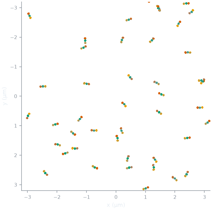
The coverslip is cut into 2 µm tiles. Each tile holds a Poisson number of candidate molecules (rods or plates; "rods" below) (mean = the density × 4 µm²; DensityPerUm2, default 1.2 µm⁻², estimate), each at a uniform position in the tile and a uniform direction. By default the rods are placed independently (a Poisson field: they may touch or cross). A minimum spacing (MinSpacingNm, default 0 = none) removes a candidate when a candidate of higher priority (a random number per candidate) lies within it, looking across the neighbouring tiles too (Matérn type II thinning): the rods left are then never closer than that, centre to centre, and the density after thinning is below the set one. The draws for the field are separate from those for the bending, so changing the persistence length, the spacing or the design never moves or turns a rod.

Bending

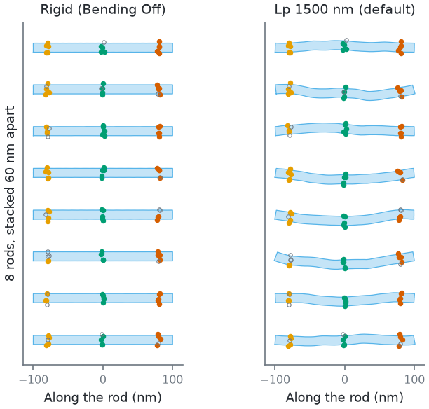
A rod lying on the glass bends within the plane. Its centreline is a two-dimensional worm-like chain: a chain that has equilibrated on the surface, as DNA can on a suitable one [rivetti1996]. The rod (L = 200 nm at the default spacing) is cut into \(n = \max\left(8, \lceil L / (D/2) \rceil\right) = 31\) segments of length \(\Delta s = L / n\). Segment j turns the direction by a normal angle step:

\[ \Delta\theta_j = z_j \sqrt{\Delta s / L_p}, \qquad z_j \sim \mathcal{N}(0, 1) \]

so the direction makes a random walk along the rod. Each segment is an exact circular arc of its own curvature, so the contour length stays L. Cross-sections stay straight and normal to the centreline: the 13 nm body is drawn around it, and a strand keeps its place along the rod and across it. The bent rod is then placed with the line between its ends along its direction and the middle of that line at its position. For this chain:

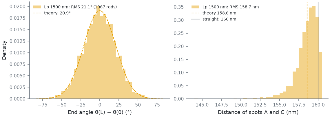
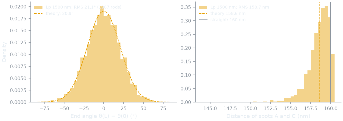
• the end tangents differ by a normal angle of variance L / L_p: 20.9° RMS at the default 1500 nm;
• the tangent correlation over a contour s is ⟨cos Δθ(s)⟩ = e^{−s / 2L_p} (the 3D chain's e^{−s / L_p}, with half the freedom to turn);
• so the mean square distance between two points s apart is the 3D chain's formula with L_p → 2L_p: ⟨R²⟩ = 4 L_p s [1 − (2L_p/s)(1 − e^{−s / 2L_p})].

The persistence length (PersistenceLengthNm, Advanced, default 1500 nm, an estimate). Measured bending persistence lengths of DNA-origami helix bundles are 740 nm to 1 µm for four-helix, 1-3 µm for six-helix and 3-8.2 µm for eight-helix bundles [chhabra2020] (their summary of the measurements, p. 4 of the arXiv version; simulations give somewhat higher values). A 12-helix rod is stiffer still, so 1500 nm leans to the soft side. Bending Off makes every rod straight.

The first 8 rods of a nanoruler field, each in its own frame (the line between its ends along x, its middle at 0) and stacked 60 nm apart: the bent 13 nm wide body (blue) and the dyes of its docking strands, coloured by spot (A, B, C at 20, 100 and 180 nm along it; hollow grey: a strand the labelling left without a dye, 80 % incorporation). The same rods, landing and labels in both: only the bending changes. Left: rigid; right: the default persistence length of 1500 nm. Each spot's five strands are a ring around the rod seen from above (a random roll per rod), so they spread across it; the dyes sit up to 3 nm (the linker) off their anchors.

How this figure was made (2 cli runs, 10 ms)

Generated by tools/build_physics_figures.py (figure ruler-shapes) from the code it documents at commit 72b1b0f, on Linux with 4 threads, 2026-11-01. Commands, in order, with their wall time (those marked [served] ran one after the other in one insiliscope_cli --serve process, which keeps the world and the PSF kernel between commands; their outputs are the same as separate runs'):

insiliscope_cli --geometry-json rigid.geometry.json --x 0 --y 0 --specimen Nanorulers --geometry-um 6 --geometry-detail 1 --origami-bend 0    # 6.1 ms [served]
insiliscope_cli --geometry-json lp1500.geometry.json --x 0 --y 0 --specimen Nanorulers --geometry-um 6 --geometry-detail 1    # 3.9 ms [served]

How far bending moves the spots: the outer spots, 160 nm apart along the rod, are 158.6 nm apart (RMS, the formula above) at 1500 nm; bending can only bring them closer.

Bending statistics of the rods in a 40 µm square, at the default persistence length of 1500 nm. Left: the angle between the two end tangents, a normal distribution of variance L/Lp (L = 200 nm) for a 2D worm-like chain. Right: the distance between the centres of the outer spots (160 nm apart along the rod); bending only shortens it. The dashed lines are the 2D chain's RMS end-to-end distance over 160 nm, √(4 Lp s [1 − (2 Lp/s)(1 − e^−s/2Lp)]) [rivetti1996]. Rods whose bend folds a cross-section over (curvature × 6.5 nm ≥ 1): 0 of them.

How this figure was made (1 cli run, 183 ms)

Generated by tools/build_physics_figures.py (figure ruler-wlc) from the code it documents at commit 72b1b0f, on Linux with 4 threads, 2026-11-01. Commands, in order, with their wall time (those marked [served] ran one after the other in one insiliscope_cli --serve process, which keeps the world and the PSF kernel between commands; their outputs are the same as separate runs'):

insiliscope_cli --geometry-json lp1500.geometry.json --x 0 --y 0 --specimen Nanorulers --geometry-um 40 --geometry-detail 1    # 183 ms [served]

A bend sharper than the half-width of the rod (curvature × 6.5 nm ≥ 1) would fold a cross-section over itself; such rods are counted (the geometry output's fold) but kept. None occur at the default persistence length.

Landing and heights

Each rod lands rolled about its own axis: a uniform random roll per rod (Roll = Uniform), or one fixed angle for all (Fixed, RollDeg). The roll turns each spot's ring of strands, so seen from above the strands of a spot lie at different places across the rod. The rod's bottom is AttachHeightNm (7 nm, estimate: the surface coating) above the glass.

The sample is two-dimensional (v1): every strand sits at the height of the rod's axis, 7 + 6.5 = 13.5 nm above the coverslip. KeepHeights (Expert) puts each strand at its ring height around the rod instead (from 7 to 20 nm), a first step towards 3D designs, not validated yet.

The label

The docking strands are the sample's one target (docking, options ruler-*, Micro-Manager Nanorulers.Docking_*). They take a label like the cell field's microtubules: a dye of the library in a mode (Dyes and light path).

• Typical labels (data/dyes/library.json typicalLabels.docking): an ATTO 655 imager in DNA-PAINT (the default), AF647 in dSTORM, mEos3.2 in PALM, ATTO 655 in WideField; the dye of a non-PAINT mode stands for a dye attached to the strand.
• Labelled % (Docking_LabelingPct, 80 %, estimate): the share of designed strands that were incorporated and carry a dye, drawn independently per strand.
• Linker (LinkerNm, 3 nm, estimate): each dye lies at a random point within this distance of its strand's anchor, on the outer side.
• DNA-PAINT: each strand binds imagers at k_on × c, with c the imager concentration in the buffer (Docking_ImagerNanoMol, Advanced, 20 nM by default: the setting for how dense the frames are), and the free imager adds a uniform background (photophysics). The binding kinetics are the docking strands' (data/specimens.json paint), not the dye's: k_on 10⁶ M⁻¹ s⁻¹ (KonPerMolarPerSec) and a bound half-time of 200 ms (mean 0.289 s, BoundTimeSec), both estimates (9 nt docking strands bind for about 0.3-1 s). A rod with 12 labelled strands then binds an imager about every 80 s per nM: every ~4 s at the default 20 nM, each binding lasting a few frames, so a field of view shows a few rods binding per frame over the free imager's background. Lower the concentration for sparser frames and less background; take thousands of frames, as in a real DNA-PAINT experiment.

The nanorulers in a 64 × 64 px field of view of 100 nm pixels (44 rods at the default 1.2 per µm²): the bent bodies and their dyes, coloured by spot as above. The spots of a rod lie 80 nm apart, less than a pixel: the camera sees each rod as one blur, and only localising the single binding events (the viewer's Localisations layer, or any SMLM software) separates them.

How this figure was made (1 cli run, 10 ms)

Generated by tools/build_physics_figures.py (figure ruler-field) from the code it documents at commit 72b1b0f, on Linux with 4 threads, 2026-11-01. Commands, in order, with their wall time (those marked [served] ran one after the other in one insiliscope_cli --serve process, which keeps the world and the PSF kernel between commands; their outputs are the same as separate runs'):

insiliscope_cli --geometry-json fov.geometry.json --x 0 --y 0 --specimen Nanorulers --geometry-um 6.4 --geometry-detail 1    # 10 ms [served]

Parameters

Viewer	Micro-Manager	CLI	Default	Source
Specimen	SampleHolder	--specimen	CellField
Design	Nanorulers.Design	--origami-design	Nanoruler	[scheckenbach2020] (body)
Site spacing	Nanorulers.SpacingNm	--origami-spacing-nm	80 nm
Density	Nanorulers.DensityPerUm2	--origami-density	1.2 µm⁻²	estimate
Strands per spot	Nanorulers.StrandsPerSpot	--origami-strands-per-spot	5	modelling choice
Bending	Nanorulers.Bending	--origami-bend	On
Persistence length	Nanorulers.PersistenceLengthNm	--origami-lp-nm	1500 nm	estimate, [chhabra2020] (range)
Min spacing	Nanorulers.MinSpacingNm	--origami-min-spacing-nm	0 (none)
Height above glass	Nanorulers.AttachHeightNm	--origami-attach-nm	7 nm	estimate
Linker	Nanorulers.LinkerNm	--origami-linker-nm	3 nm	estimate
Roll, roll angle	Nanorulers.Roll, RollDeg	--origami-roll, --origami-roll-deg	Uniform, 0°
3D strand heights	Nanorulers.KeepHeights	--origami-heights	Off
Docking strands label	Nanorulers.Docking_Label, _Mode, _LabelingPct, _ImagerNanoMol	--ruler-dye, --ruler-mode, --ruler-label-pct, --ruler-imager-nm	Typical (ATTO 655 DNA-PAINT), 80 %, 20 nM	estimates
DNA-PAINT binding	Nanorulers.Docking_BoundTimeSec, _KonPerMolarPerSec	--ruler-paint-on-sec, --ruler-paint-kon	0.289 s (half-time 200 ms), 10⁶ M⁻¹s⁻¹	estimates

The core parameters are the origami* names (origamiLpNm, ...; p.<name> on the CLI). The CLI's --geometry-json lists each molecule in a window (position, direction, roll, end angle, fold, the bent outline and, with --geometry-detail 1, every strand: spot, ring position, world position, straight and bent position in the molecule's frame, labelled or not); the figures on this page are made from it.

Limits

• Two-dimensional: the molecules lie flat, the strands at one height; no 3D designs yet. 2D origami land face up only (a sheet that lands face down would show its pattern mirrored, with the strands under it).
• Every rod is whole: no broken rods, missing spots or misfolded molecules beyond the labelled %.
• Uniform stiffness, no built-in curvature; rods may touch or cross (a minimum spacing thins them by their centres only).
• Bodies: a cylinder with in-plane bending (or none) and a uniform or fixed roll, and a rigid plate with a hex map of strands.
• No BrightField contrast (see Samples).
• The viewer draws the rods in its map; its animation exports do not include them yet.