Structures

Each cell is generated in its own local frame (origin at the cell centre, units um, \(z\) = height above the coverslip) and mapped to the world by the cell's packing rotation and position.

Nucleus

A shaped ellipsoid per cell: long axis, short/long ratio and height (as a fraction of the long axis) are drawn from ranges (defaults, all estimates: long axis 8-12 µm, ratio 0.6-1, height 0.2-0.3 of the long axis). Nucleus size is correlated with cell size by reusing the same hash draw (same percentile of both ranges), and offset from the cell centroid by up to a fraction of the cell radius.

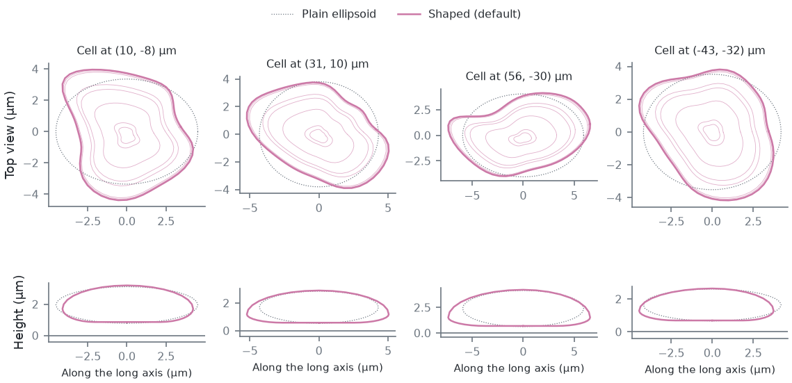
Real nuclei are not ellipsoids: their outlines are smooth egg, bean or rounded-triangle shapes with radius deviations of a few to ~10 %, and adherent nuclei are wider at the base (estimates from images; no measured shape distribution is used). Each nucleus therefore gets, from its own hash stream (every default below an estimate):

• lobes: the footprint radius is \(1 + \sum_{k=2}^{8} (a_k \cos k\theta + b_k \sin k\theta)\) (soft-clamped), with a \(k^{-\gamma}\) spectrum (nucSmooth, default 2.5) normalised so the rms relative deviation is the cell's irregularity (nucIrregMin-nucIrregMax, default 0.03-0.2);
• a kidney bend (nucBendMin-nucBendMax, 0-0.3): an invertible shear of the outline;
• an uneven thickness (nucThickIrreg, 0.1 rms at the edge);
• a wider base (nucAsym, 0.5: sections below the widest one are widened toward it; negative values widen the top) and a lowered widest point (nucWidestMin-nucWidestMax, 0.2-0.4 of the height above the bottom).

All shape terms at 0 (and the widest point at 0.5) give the plain ellipsoid. The nucleus sits on a thin basal layer of cytoplasm: its bottom is nucBaseMin-nucBaseMax (0.4-0.9 µm, estimate) above the coverslip, and the dome top follows the nucleus top plus the margin (nucMargin, 0.5 µm, estimate). A lateral envelopment step keeps the whole footprint inside the cell outline with that margin.

In Micro-Manager these are the CellField.Nuc* properties (NucBaseMinUm/MaxUm, NucIrregMin/Max, NucBendMin/Max, NucSmooth, NucThickIrreg, NucAsym, NucWidestMin/Max); in the cli and viewer, p.<name>.

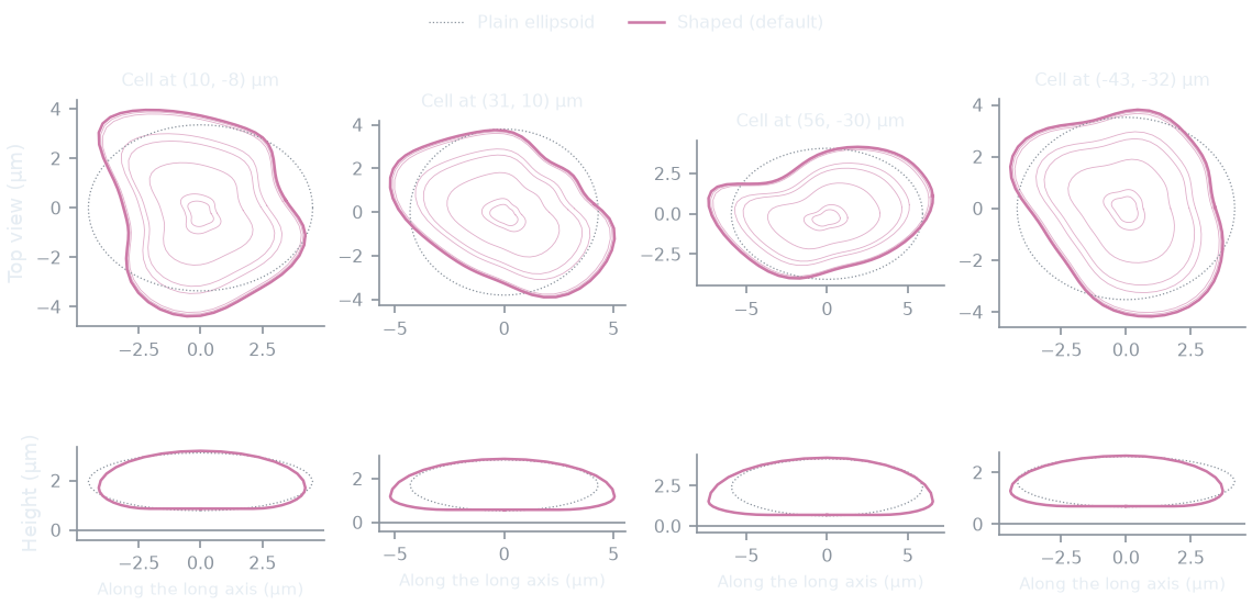
Shaped nuclei next to the plain ellipsoids the same cells would have with every shape term at 0:

The nuclei of the four cells nearest the figures' spot (seed 42). Top: in each nucleus's own frame (long axis horizontal), the widest section and, faint, every third section. Bottom: the silhouette seen from the side. Pink: the shaped nucleus (defaults: lobes, kidney bend, uneven thickness, wider base, lowered widest point); dotted grey: the same cell with every shape term at 0, the plain ellipsoid. The line at height 0 is the coverslip: the nucleus sits on a basal layer of cytoplasm.

How this figure was made (2 cli runs, 331 ms)

Generated by tools/build_physics_figures.py (figure struct-nucleus) from the code it documents at commit 72b1b0f, on Linux with 4 threads, 2026-11-01. Commands, in order, with their wall time (those marked [served] ran one after the other in one insiliscope_cli --serve process, which keeps the world and the PSF kernel between commands; their outputs are the same as separate runs'):

insiliscope_cli --geometry-json shaped.geometry.json --nucleus-json shaped.nuclei.json --x 6.58 --y -5.61 --geometry-um 70 --geometry-detail 0 --npc-dye None    # 42 ms [served]
insiliscope_cli --geometry-json plain.geometry.json --nucleus-json plain.nuclei.json --x 6.58 --y -5.61 --geometry-um 70 --geometry-detail 0 --p.nucIrregMin 0 --p.nucIrregMax 0 --p.nucBendMax 0 --p.nucThickIrreg 0 --p.nucAsym 0 --p.nucWidestMin 0.5 --p.nucWidestMax 0.5 --npc-dye None    # 289 ms [served]

Cytoplasm

A height field over the cell footprint: dome over the nucleus (slope capped, cytoDomeSlope), a saturating rise from the edge, Hc(1 - e^{-s d_{edge}/Hc}) with \(H_c = 2 h_{mid}\), so the cell never has a linear pyramid flank. Defaults (estimates; the viewer's "Rounded" look since 2026-10-03): rim height 0.2-0.5 µm, mid height 2-3.5 µm, slope caps 2 (cytoplasm) and 4 (dome); the viewer's Cell look presets set other profiles. 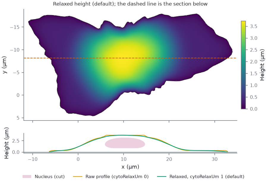That raw profile is a min/max of distance fields and has creases ("folds"), so the height is relaxed: on a 0.25 µm grid it solves \(h - \ell^2 \nabla^2 h = h_{raw}\) (\(\ell\) = cytoRelaxUm, default 1 µm, an estimate), a membrane under tension pulled toward the profile, with \(h = 0\) on the exact outline and \(h \ge\) nucleus top + margin over the nucleus. Microtubules, dyes and the brightfield volume all use this relaxed height, not the raw analytic one.

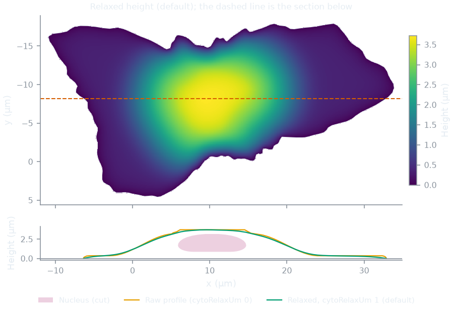
The raw and the relaxed height of one cell:

The cytoplasm height of the cell nearest the spot, from the core's mesh (the BrightField volume, microtubules and dyes use the same height). Below: the section along the dashed line through the nucleus centre, at the same scale as the map (cells are flat). The raw profile (a min/max of distance fields) has creases where its pieces meet; the relaxed one solves h - l²∇²h = h_raw on a 0.25 µm grid, with h = 0 on the outline and at least the nucleus top plus its margin over the nucleus.

How this figure was made (2 cli runs, 889 ms)

Generated by tools/build_physics_figures.py (figure struct-cytoplasm) from the code it documents at commit 72b1b0f, on Linux with 4 threads, 2026-11-01. Commands, in order, with their wall time (those marked [served] ran one after the other in one insiliscope_cli --serve process, which keeps the world and the PSF kernel between commands; their outputs are the same as separate runs'):

insiliscope_cli --geometry-json relaxed.geometry.json --nucleus-json relaxed.nuclei.json --x 6.58 --y -5.61 --geometry-um 2 --geometry-detail 1 --npc-dye None    # 316 ms [served]
insiliscope_cli --geometry-json raw.geometry.json --nucleus-json raw.nuclei.json --x 6.58 --y -5.61 --geometry-um 2 --geometry-detail 1 --p.cytoRelaxUm 0 --npc-dye None    # 573 ms [served]

Microtubules

Each microtubule is a 3D path from near the nucleus to near the cell edge:

1. Start: a point of the cytoplasm volume with density \(\propto e^{-d/\lambda}\), \(d\) the distance to the nucleus surface and \(\lambda\) = mtStartDecayPct (1.6 %, estimate) of the cell's equivalent diameter (~0.5 µm).
2. End: twelve candidate points of the footprint outside the nucleus, density \(\propto e^{-d/\lambda}\) with \(d\) the distance to the outline (mtEndDecayPct, 20 %, ~6 µm, estimate); one is picked with weight \(e^{\kappa(\cos a - 1)}\), \(a\) the angle between start-to-end and the outward direction at the start (mtDirKappa, 1.5, estimate; 0 = any direction, so paths also cross over or under the nucleus). Micro-Manager: CellField.MicrotubuleStartDecayPct, ...EndDecayPct, ...DirKappa.
3. Path: a correlated random walk in \(xy\) with a bounded turn radius, forced onto both endpoints with a Brownian-bridge drift correction. The persistence length is shared between the heading walk and \(z\), implemented so that the correlation length is fixed in real um regardless of step length (a discretised Ornstein-Uhlenbeck process in arc length; the heading kick scales as \(\sqrt{\ell_{step}/\ell_{corr}}\), the worm-like-chain relation). The correlation length (mtSmoothLen, default 1.5 µm) is an estimate for microtubules in cells, far below the thermal persistence length of taxol-stabilized microtubules in vitro, 5.2 mm [gittes1993].
4. Height is a fraction of the local cytoplasm ceiling, interpolated between start and end and converted using the ceiling at each point, so paths ride the actual slope, then box-smoothed. Where a path crosses the nucleus it rides over (or, starting low, under) it with a clearance, lifted or lowered by a smooth ramp rather than point by point (a generic obstacle interface: the nucleus is the first obstacle). A slope cap removes residual jitter.
5. Points are kept inside the cell volume; the walk is truncated at the first exit from the footprint (no edge hugging); a bounded minimum-separation pass separates microtubules in 3D.

Density is given per µm\(^2\) of cell footprint (default 0.9/µm\(^2\), an estimate).

The microtubules of one cell from above and from the side, and with the direction preference switched off:

Microtubule centrelines of the cell nearest the spot, coloured by height: 47 of its 560 shown. Top: with the default direction weight the paths run outward from near the nucleus; with mtDirKappa 0 the end point ignores direction and paths also cross over the nucleus. Bottom: the default paths seen from the side, each a fraction of the local cytoplasm ceiling, over (or, starting low, under) the nucleus.

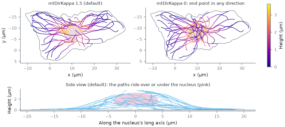
How this figure was made (2 cli runs, 647 ms)

Generated by tools/build_physics_figures.py (figure struct-microtubules) from the code it documents at commit 72b1b0f, on Linux with 4 threads, 2026-11-01. Commands, in order, with their wall time (those marked [served] ran one after the other in one insiliscope_cli --serve process, which keeps the world and the PSF kernel between commands; their outputs are the same as separate runs'):

insiliscope_cli --geometry-json default.geometry.json --nucleus-json default.nuclei.json --x 6.58 --y -5.61 --geometry-um 2 --geometry-detail 1 --npc-dye None    # 316 ms [served]
insiliscope_cli --geometry-json kappa0.geometry.json --nucleus-json kappa0.nuclei.json --x 6.58 --y -5.61 --geometry-um 2 --geometry-detail 1 --p.mtDirKappa 0 --npc-dye None    # 331 ms [served]

Fluorophore sites (dye lattice)

A microtubule is a 25 nm cylinder [mikhaylova2015, weber1978] carrying the 13_3 protofilament lattice: 13 protofilaments [tilney1973], protofilament \(k\) at angle \(\phi_0 + 2\pi k/13\) and axial offset \((3 k \cdot 8/13) \bmod 8\) nm, a site every 8 nm dimer (about 1625 sites per µm). In the measured B-lattice the 4 nm monomers lie on a 3-start helix, so neighbouring protofilaments are staggered by 12 nm/13 = 0.92 nm and the lattice has a seam [mandelkow1986]; the model's 1.85 nm step (3 dimers per turn) closes without a seam, a simplification that keeps the sites per µm.

quantity	value
attachment radius	12.5 nm from the axis (half the 25 nm diameter [mikhaylova2015])
binder (nanobody/antibody) stalk	12 nm radially outward (estimate)
dye displacement from the binder tip	uniform in volume, 2-5 nm, uniform direction (linker; estimate)

Stalk plus linker widen a labelled microtubule by up to 34 nm (2 x (12 + 5) nm), within the 20-40 nm of common labels [mikhaylova2015]; primary plus secondary antibodies take it from 25 to about 60 nm [weber1978], nanobodies add less [mikhaylova2015].

Sites are never materialised for a whole field. A dye's identity is a hash of (cell, microtubule, protofilament, dimer); whether it is labelled, whether it ever activates and what it does are decided from hashes first, and 3D positions are only computed for dyes that will emit. The unit of generation is a block: 1 µm of one microtubule.

The lattice as the core generates it, read back through the cli's dye-site output:

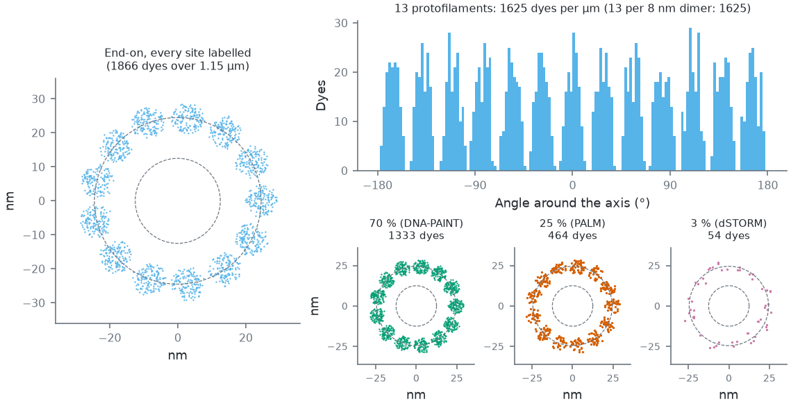
Dye positions on a 1.2 µm piece of one microtubule, from the core's site query (each site's offset from the centreline). End-on, the dyes form a ring: the 12.5 nm lattice radius [mikhaylova2015] (inner dashed circle) plus the 12 nm binder (outer; estimate), spread by the 2-5 nm linker (estimate): the Legacy linkage (mt-binder Legacy; the default IgG2-PAINT puts the dyes on a wider, softer shell, below); measured radius 24.6 ± 2.3 nm. Around the axis: 13 peaks, one per protofilament [tilney1973], widened by the linker. Bottom: the same piece end-on at each mode's typical labelled share (the sites that carry a dye).

How this figure was made (5 cli runs, 1.25 s)

Generated by tools/build_physics_figures.py (figure struct-lattice) from the code it documents at commit 72b1b0f, on Linux with 4 threads, 2026-11-01. Commands, in order, with their wall time (those marked [served] ran one after the other in one insiliscope_cli --serve process, which keeps the world and the PSF kernel between commands; their outputs are the same as separate runs'):

insiliscope_cli --geometry-json geo.geometry.json --nucleus-json geo.nuclei.json --x 6.58 --y -5.61 --geometry-um 2 --geometry-detail 1 --npc-dye None    # 428 ms [served]
insiliscope_cli --dyes-json pct100.dyes.json --x 6.58 --y -5.61 --mt-label-pct 100 --mt-binder Legacy --dyes-rect 16.3915,-5.0142,17.7003,-4.3736 --dyes-z -0.0768,0.0912 --dyes-t 60,60.05 --npc-dye None    # 207 ms [served]
insiliscope_cli --dyes-json pct70.dyes.json --x 6.58 --y -5.61 --mt-label-pct 70 --mt-binder Legacy --dyes-rect 16.3915,-5.0142,17.7003,-4.3736 --dyes-z -0.0768,0.0912 --dyes-t 60,60.05 --npc-dye None    # 208 ms [served]
insiliscope_cli --dyes-json pct25.dyes.json --x 6.58 --y -5.61 --mt-label-pct 25 --mt-binder Legacy --dyes-rect 16.3915,-5.0142,17.7003,-4.3736 --dyes-z -0.0768,0.0912 --dyes-t 60,60.05 --npc-dye None    # 205 ms [served]
insiliscope_cli --dyes-json pct3.dyes.json --x 6.58 --y -5.61 --mt-label-pct 3 --mt-binder Legacy --dyes-rect 16.3915,-5.0142,17.7003,-4.3736 --dyes-z -0.0768,0.0912 --dyes-t 60,60.05 --npc-dye None    # 205 ms [served]

Labelling. Each structure carries one label (issue 16): a share of its sites (density, cli/viewer mt-label-pct / npc-label-pct, MM CellField.Microtubules_LabelingPct / NuclearPores_LabelingPct) carries a dye. One LABEL draw per site, \(u < \) density, picks them (the same threshold as before, so a density equal to the old bleaching + persistent fractions gives the same dyes); a second, nested FLUOR draw keeps the dye's fluorescent fraction (none at fraction 1). What the dyes do depends on the label's mode (dSTORM, PALM, DNA-PAINT, WideField): Photophysics. Each dye also has an orientation (free, fixed or random, with a wobble cone; its own draws), not used by the renderer yet. Default: DNA-PAINT on 70% of the sites (an estimate).

Nuclear pore complexes

The cell field's second target (2026-10-12), labelled and imaged together with the microtubules. Each pore is the Nup96 model of webSMLM [thevathasan2019]: two rings 50 nm apart along the pore axis (the cytoplasmic one outside the nucleus, the nucleoplasmic one inside), eight corners per ring at a radius of 53.5 nm, four attachment points per corner on an arc 12 nm across, so 64 sites per pore.

• Where. Pores cover the whole nuclear envelope, uniformly by area (a fixed triangle mesh of the shaped nucleus picks the place, which is then put exactly on the membrane), each along the local outward normal with a random twist about it, so pores at the bottom of the nucleus are seen from below and those on its flanks from the side.
• How many. npc-density (MM CellField.NuclearPoreDensityPerUm2, Advanced) per µm² of envelope, default 8: the count is that times the envelope's area, rounded, so a lower density keeps a subset of the same pores. Measured interphase densities are 5-9 per µm² [maeshima2006, dultz2010]. A new pore closer than npcMinDistNm (MM CellField.NuclearPoreMinDistNm, Expert; default 180 nm, a pore being about 120 nm across) to one already placed is redrawn.
• Label. Default DNA-PAINT with a Cy3B imager at 561 nm on 60% of the sites: 2.5 nM (npc-imager-nm, MM NuclearPores_ImagerNanoMol; estimate, the microtubules' is 1 nM), binding as the microtubules' imager does (k_on 10⁶ M⁻¹ s⁻¹, mean bound time 0.05 s, estimates; npc-paint-kon, npc-paint-on-sec, MM NuclearPores_KonPerMolarPerSec, _BoundTimeSec); the typical labels per mode follow the pore literature (dSTORM: Nup96-SNAP + BG-AF647, 58%; PALM mEos3.2; WideField mEGFP) [thevathasan2019, schlichthaerle2019]. Set the pore label to None (npc-dye None) to image the microtubules alone, as before.
• Brightfield. Pores add no brightfield contrast (sub-resolution, far below the cell's phase).

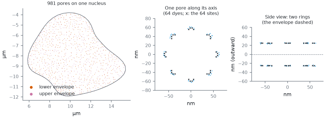
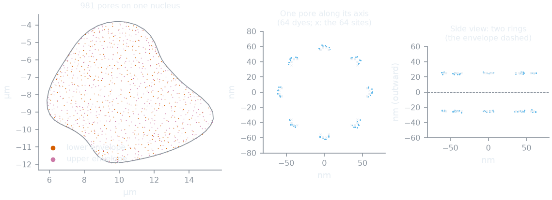
Nuclear pores from the core (--geometry-json with detail, --dyes-json). Left: one cell's pores (8 per µm² of envelope and at least 180 nm apart, the defaults) over its nucleus, uniform by area over the whole envelope; the lower envelope is the one near the coverslip. Middle and right: the dyes of its most downward-facing pore with every site labelled, in the pore's frame: 8 corners of 2 x 4 sites per ring at 53.5 nm (Nup96 [thevathasan2019]), the cytoplasmic ring 25 nm outside the envelope, the nucleoplasmic one 25 nm inside; the default SNAP-Halo linkage spreads them by a few nm (dye radius 60.1 ± 1.9 nm).

How this figure was made (2 cli runs, 520 ms)

Generated by tools/build_physics_figures.py (figure struct-npc) from the code it documents at commit 72b1b0f, on Linux with 4 threads, 2026-11-01. Commands, in order, with their wall time (those marked [served] ran one after the other in one insiliscope_cli --serve process, which keeps the world and the PSF kernel between commands; their outputs are the same as separate runs'):

insiliscope_cli --geometry-json geo.geometry.json --nucleus-json geo.nuclei.json --x 6.58 --y -5.61 --geometry-um 2 --geometry-detail 1 --npc-dye None    # 313 ms [served]
insiliscope_cli --dyes-json pore.dyes.json --x 6.58 --y -5.61 --mt-dye None --npc-label-pct 100 --dyes-rect 8.2166,-8.9559,8.4566,-8.7159 --dyes-z 0.6637,0.9037 --dyes-t 60,60.05    # 207 ms [served]

Nuclear lamina

The cell field's third target (2026-10-27), unlabelled by default: it shows only once you give it a dye. For now a random stand-in for the lamin network under the nuclear envelope: points, not filaments.

• Where. Points cover the whole nuclear envelope, uniformly by area and independently of each other (the pores' mesh picks the place, which is then put exactly on the membrane), but none within 20 nm of a pore's centre: a disc of p.laminNpcExclNm (MM CellField.NuclearLaminaPoreExclusionNm, Expert; default 40 nm, estimate) across around every pore, whether the pores are labelled or not.
• How many. lamin-density (MM CellField.NuclearLaminaDensityPerUm2, Advanced; 100 to 10 000 in the viewer and Micro-Manager) per µm² of envelope, default 2000 (estimate): the count is that times the envelope's area, rounded (some 250 000 on a nucleus of ~125 µm²). The viewer's View > Nuclear lamina draws the envelope they lie on as a surface, not the points one by one, its opacity following their local density.
• Label. One docking site per point, labelled through the same path as the other targets (lamin-dye, lamin-mode, lamin-label-pct, lamin-imager-nm, the linkage lamin-binder*; MM NuclearLamina_*). The linkage starts at the point in a random direction (every direction equally likely, no side of the envelope preferred); default anti-lamin primary + secondary antibodies (IgG2-PAINT). The typical labels per mode (DNA-PAINT Cy3B 70%, dSTORM AF647 70%, PALM mEos3.2 58%, WideField mEGFP 100%) and the DNA-PAINT binding (2.5 nM imager, the pores' k_on and bound time) are estimates. To turn it on: lamin-dye Typical on the cli, the Dye select of the Nuclear lamina label group in the viewer, CellField.NuclearLamina_Label in Micro-Manager.
• Brightfield. No brightfield contrast.

Label linkage: where the dye sits

A dye does not sit on its structure: a probe holds it there. One model for every target: the binder (the probe: primary + secondary antibodies, a nanobody, a SNAP or Halo tag, a fusion protein, a docking strand) points away from the structure (radially from a microtubule, from a pore's corner outwards, from a lamina point in a random direction) by its length, with a flexibility (a random offset in a ball); then a short chemical linker in a random direction; then the dye. Presets (cli/viewer <prefix>-binder, MM <Target>_Binder, Advanced; the numbers in Expert) come from measured label shells [fruh2021, nieves2019]. Defaults: the microtubules through primary + secondary antibodies (IgG2-PAINT: the dyes on a shell ~32 nm from the axis around the 12.5 nm tube, as measured for DNA-labelled secondaries), the pores on a SNAP/Halo tag (a few nm). Legacy keeps the numbers from before the presets (12 nm + a 2-5 nm linker on a microtubule).

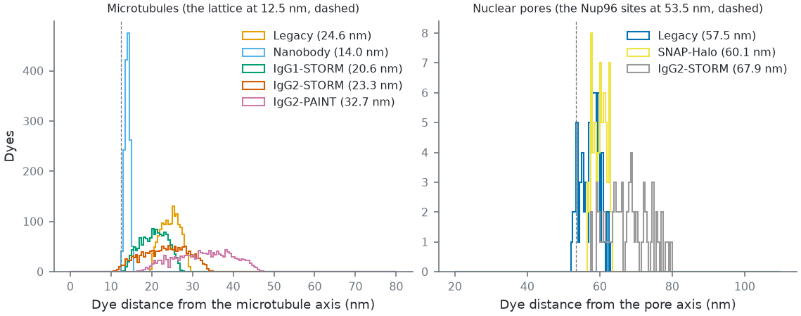
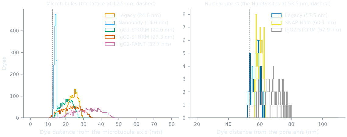
Where the dyes sit under the label linkage presets (mt-binder, npc-binder; MM <Target>_Binder), every site labelled, from the core's site query. Antibody shells after [fruh2021] Table 1 (the IgG2-PAINT shell, 31.8 nm, is wider than with a dye: partly unfolded DNA-antibody conjugates, the authors suspect), the nanobody after [mikhaylova2015], SNAP/Halo after [nieves2019]; Legacy = the numbers before the presets. Defaults: microtubules IgG2-PAINT, pores SNAP-Halo. On a pore, antibodies widen the ring as measured (64.3 vs 53.7 nm with SNAP [thevathasan2019]).

How this figure was made (9 cli runs, 1.96 s)

Generated by tools/build_physics_figures.py (figure struct-linkage) from the code it documents at commit 72b1b0f, on Linux with 4 threads, 2026-11-01. Commands, in order, with their wall time (those marked [served] ran one after the other in one insiliscope_cli --serve process, which keeps the world and the PSF kernel between commands; their outputs are the same as separate runs'):

insiliscope_cli --geometry-json geo.geometry.json --nucleus-json geo.nuclei.json --x 6.58 --y -5.61 --geometry-um 2 --geometry-detail 1 --npc-dye None    # 316 ms [served]
insiliscope_cli --dyes-json mt-Legacy.dyes.json --x 6.58 --y -5.61 --mt-label-pct 100 --mt-binder Legacy --dyes-rect 16.4539,-4.9991,17.5888,-4.3965 --dyes-z -0.0968,0.1082 --dyes-t 60,60.05 --npc-dye None    # 200 ms [served]
insiliscope_cli --dyes-json mt-Nanobody.dyes.json --x 6.58 --y -5.61 --mt-label-pct 100 --mt-binder Nanobody --dyes-rect 16.4539,-4.9991,17.5888,-4.3965 --dyes-z -0.0968,0.1082 --dyes-t 60,60.05 --npc-dye None    # 192 ms [served]
insiliscope_cli --dyes-json mt-IgG1-STORM.dyes.json --x 6.58 --y -5.61 --mt-label-pct 100 --mt-binder IgG1-STORM --dyes-rect 16.4539,-4.9991,17.5888,-4.3965 --dyes-z -0.0968,0.1082 --dyes-t 60,60.05 --npc-dye None    # 208 ms [served]
insiliscope_cli --dyes-json mt-IgG2-STORM.dyes.json --x 6.58 --y -5.61 --mt-label-pct 100 --mt-binder IgG2-STORM --dyes-rect 16.4539,-4.9991,17.5888,-4.3965 --dyes-z -0.0968,0.1082 --dyes-t 60,60.05 --npc-dye None    # 209 ms [served]
insiliscope_cli --dyes-json mt-IgG2-PAINT.dyes.json --x 6.58 --y -5.61 --mt-label-pct 100 --mt-binder IgG2-PAINT --dyes-rect 16.4539,-4.9991,17.5888,-4.3965 --dyes-z -0.0968,0.1082 --dyes-t 60,60.05 --npc-dye None    # 208 ms [served]
insiliscope_cli --dyes-json npc-Legacy.dyes.json --x 6.58 --y -5.61 --mt-dye None --npc-label-pct 100 --dyes-rect 8.2166,-8.9559,8.4566,-8.7159 --dyes-z 0.6637,0.9037 --dyes-t 60,60.05 --npc-binder Legacy    # 209 ms [served]
insiliscope_cli --dyes-json npc-SNAP-Halo.dyes.json --x 6.58 --y -5.61 --mt-dye None --npc-label-pct 100 --dyes-rect 8.2166,-8.9559,8.4566,-8.7159 --dyes-z 0.6637,0.9037 --dyes-t 60,60.05 --npc-binder SNAP-Halo    # 209 ms [served]
insiliscope_cli --dyes-json npc-IgG2-STORM.dyes.json --x 6.58 --y -5.61 --mt-dye None --npc-label-pct 100 --dyes-rect 8.2166,-8.9559,8.4566,-8.7159 --dyes-z 0.6637,0.9037 --dyes-t 60,60.05 --npc-binder IgG2-STORM    # 210 ms [served]

Adding the missing structures

A lamin network (beyond the random lamina points above), mitochondria, DNA and other cell types are not implemented yet; see Extending for how a new per-cell generator keyed off the same (seed, address, channel) scheme plugs in.

Further details and the history of each fix: spec/ALGORITHM.md.